Machine Learning: Linear Regression, Simply Explained

Linear regression is fitting a line to our data.
First, let's explore linear regression when we have only one variable (one feature; one independent variable).
Suppose that we have a table that describes house prices based on one feature which is the size of the house:
| Size in m2 (x) | Price in $ (y) |
|---|---|
| 2104 | 460,000 |
| 1416 | 232,000 |
| 1002 | 112,000 |
| 1721 | 382,000 |
| 1590 | 266,000 |
| 1302 | 201000 |
Let \(m\) be the number of examples, \(x^i\) be the i-th element for variable \(x\) , and \(y^i\) be the i-th element for variable \(y\). For our example, \(m=4\), \(x^2=1416\), and \(y^3=112,000\). In real cases, \(m\) is much large than 4. We use four entries here just for clarification.
The variable \(x\) is called feature, and variable \(y\) is called target.
We call these examples the training examples, meaning that they are used to train a machine-learning model (in our case, linear regression) so we can use that model to predict the target variable for new data.
To do so, we need to calculate a function called the hypothesis (\(h_\theta(x)\)) that can be used to predict house price knowing its size. This function has the following form:
$$ h_\theta(x)=\theta_0+\theta_1x $$
Note that this equation looks like the line equation (\(y=b+mx\)) where \(m\) is the slope of the line and \(b\) is the where the line intersects with the y axis.
In our equation, \(x\) is our one feature, the size of the house. \(\theta_0\) and \(\theta_1\) are unknowns; we need to find the optimal values for these two parameters. \(h_\theta(x)\) represents the predicted price. We want \(h_\theta(x)\) to be a good predictor, we want its value to be as close as possible to the actual \(y\) value.
Let's suppose that we have these data points:
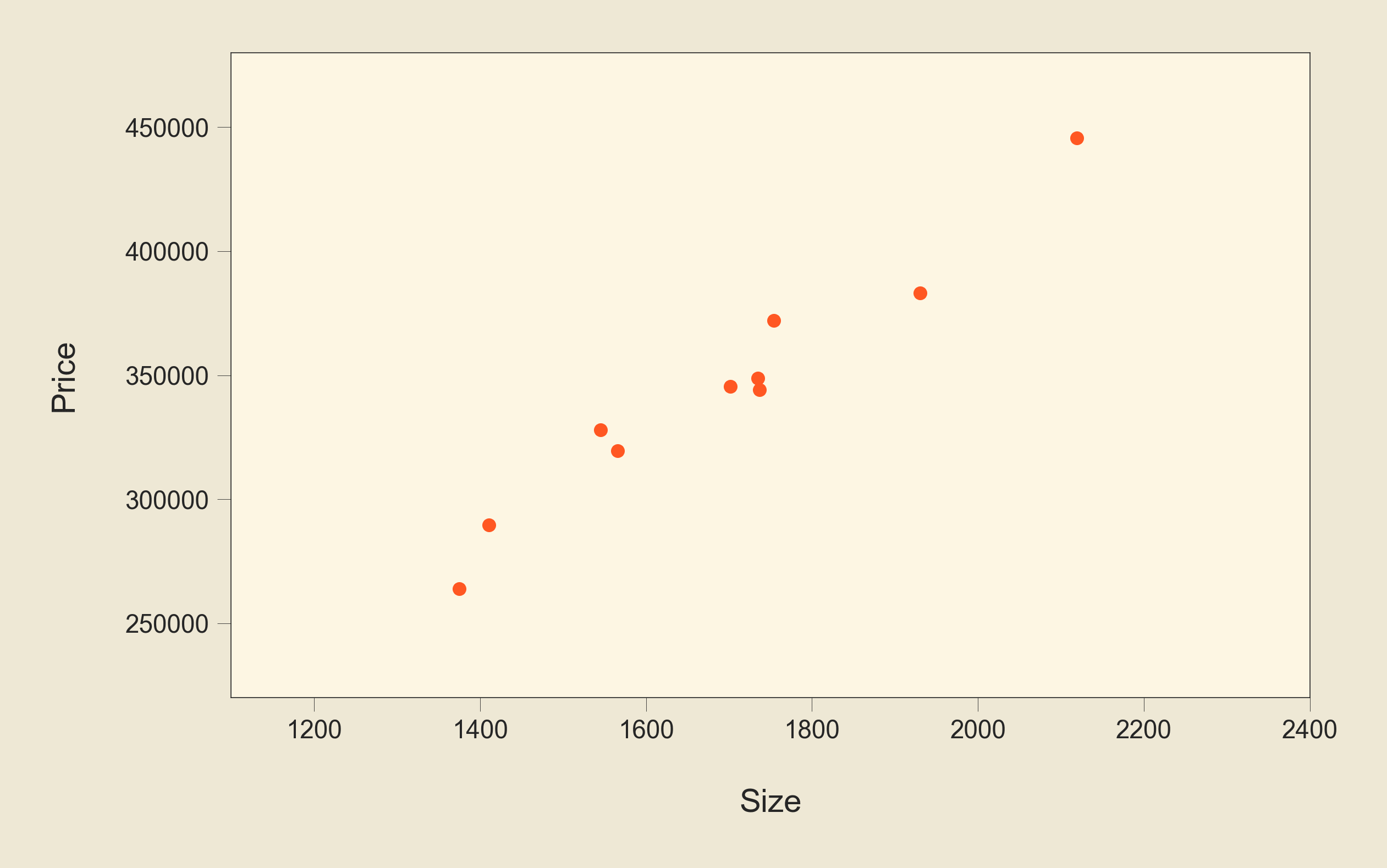
where each point represents a house, where the size of this house is on the x-axis and its price is on the y-axis.
We want to find a line that fit this data better than any other line. In other words, we want to find the optimal values for \(\theta_0\) and \(\theta_1\) in the following equation:
$$ h_\theta(x)=\theta_0+\theta_1x $$
which represents a line as we said earlier. We can try many values for \(\theta_0\) and \(\theta_1\) until we reach a satisfactory results, but this is not a practically efficient way. Instead, we will use a function called the cost function with an algorithm called gradient descent to reach the optimal values for our two parameters.
The cost function is used to calculate the error in our model, to know, for given values of \(\theta_0\) and \(\theta_1\), how good is our hypothesis, how close are the predicted values to the actual values. The cost function for linear regression can have the following formula:
$$ \text{Cost}=J(\theta)=\frac{1}{2m}\sum_{i=1}^m(h_\theta(x^i)-y^i)^2 $$
So this cost function calculates the difference between the predicted value and the actual value for all the training examples that we have. Our goal is to choose values for theta0 and theta1 that minimize the cost function.
For example, let's calculate the cost function value for the training examples in the table above, assuming that theta0=1 and theta1=2 (This is just random. We will see later how to get the optimal values for theta0 and theta1):
$$ J(\theta)=\frac{1}{2\times6}\sum_{i=1}^m(\theta_0+\theta_1x^i-y^i)^2=\\~\\\frac{1}{12}[(1+2\times2104-460000)^2+\\~\\(1+2\times1416-232000)^2+\\~\\(1+2\times1002-112000)^2+\\~\\(1+2\times1721-382000)^2+\\~\\(1+2\times1590-266000)^2+\\~\\(1+2\times1302-201000)^2] $$
Now how to choose theta values? We do so using Gradient Descent algorithm, which is the repeat of:
$$ \theta_j:=\theta_j-\alpha\frac{\partial}{\partial\theta_j}J(\theta) \qquad\text{ for }j=0,1 $$
until convergence.
:= means that we compute the right side and assign it to the left side. \(\alpha\) is the learning rate, it controls the step size of gradient descent. \(\frac{\partial}{\partial\theta_j}J(\theta)\) is the partial derivative of the cost function with respect to \(\theta_j\).
Gradient descent algorithm starts with random values of thetas. It calculates the right side of the assignment for all thetas then updates all thetas simultaneously. This happens because to calculate the right side of the assignment for some \(\theta\), you need the values of other thetas:
$$ \theta_j:=\theta_j-\alpha\frac{\partial}{\partial\theta_j}\left(\frac{1}{2m}\sum_{i=1}^m(h_\theta(x^i)-y^i)^2\right)=\\~\\\theta_j-\alpha\frac{\partial}{\partial\theta_j}\left(\frac{1}{2m}\sum_{i=1}^m(\theta_0+\theta_1x^i-y^i)^2\right) $$
The partial derivative of the cost function gives us the direction in which the gradient descent should move toward the optimal point at which the cost function has its smallest value. The partial derivative also has a magnitude that decreases as we get close to the optimal point.
So gradient descent algorithm iterates and continues updating the parameters (thetas) until convergence, until the cost function value is not decreasing anymore. At that point, we can say that the values of thetas are optimal, meaning they produce the smallest cost (error) function value. This means that we can now use the equation:
$$ h_\theta(x)=\theta_0+\theta_1x $$
to get the predicted value (\(h_\theta(x)\)) for an input value (\(x\)). Let's say that we trained the model and got the optimal values for thetas, and that we got thete0 = 1 and theta1 = 212. Now, we want to predict the price of a new house whose size is 1333 m2, we apply our model (the hypothesis):
$$ h_\theta(x)=\theta_0+\theta_1x = 1+212\times1333=282597 $$
So we got a predicted value of $ 282597 for the house price.
Multivariate linear regression
Until now, we have been talking about linear regression with one input variable (one feature). In real-world problems, there are much more features. Data for multivariate linear regression might look like:
| Size in m2 (x1) | Number of Bedrooms (x2) | Number of Floors (x3) | Age in years (x4) | Price in $ (y) |
|---|---|---|---|---|
| 2104 | 3 | 2 | 40 | 460,000 |
| 1416 | 1 | 1 | 42 | 232,000 |
| 1002 | 1 | 1 | 31 | 112,000 |
| 1721 | 2 | 2 | 22 | 382,000 |
| 1590 | 2 | 1 | 45 | 266,000 |
| 1302 | 1 | 1 | 44 | 201000 |
Here \(x_1\) is the first feature, \(x_2\) is the second one, and so on. \(x_2^1\) in this case represents the first value of the second feature (number of bedrooms), which is 3.
The number of features is denoted by \(n\). In our example, \(n\) is 4.
The same techniques used with univariate linear regression (linear regression with one variable) are used with multivariate linear regression. The difference is that we just add the new input variables with their corresponding parameters.
So, the hypothesis function becomes:
$$ h_\theta(x)=\theta_0+\theta_1x_1+\theta_2x_2+\theta_3x_3 + \cdots +\theta_nx_n $$
The cost function retain its general form:
$$ \text{Cost}=J(\theta)=\frac{1}{2m}\sum_{i=1}^m(h_\theta(x^i)-y^i)^2$$
but \(h_\theta(x)\) will make it different. Also, gradient descent becomes:
$$ \theta_j:=\theta_j-\alpha\frac{\partial}{\partial\theta_j}J(\theta) \qquad\text{ for }j=0,1,2,\cdots,n $$
Illustrated Example with Simple Python Code
Let's say that we have these data points as our training data:
Now, we want to fit a line to this data so we can use it to predict the output value for new data. First let's see a bad example of such a line:
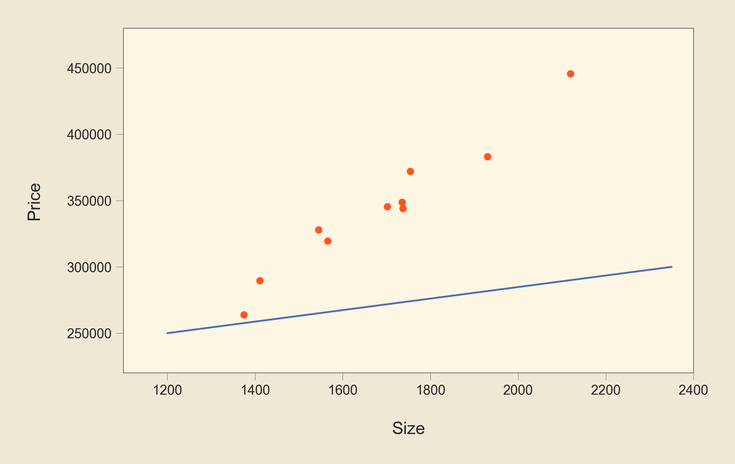
This line clearly is not the best fit. All points are on one of its sides. Let's see a better solution:
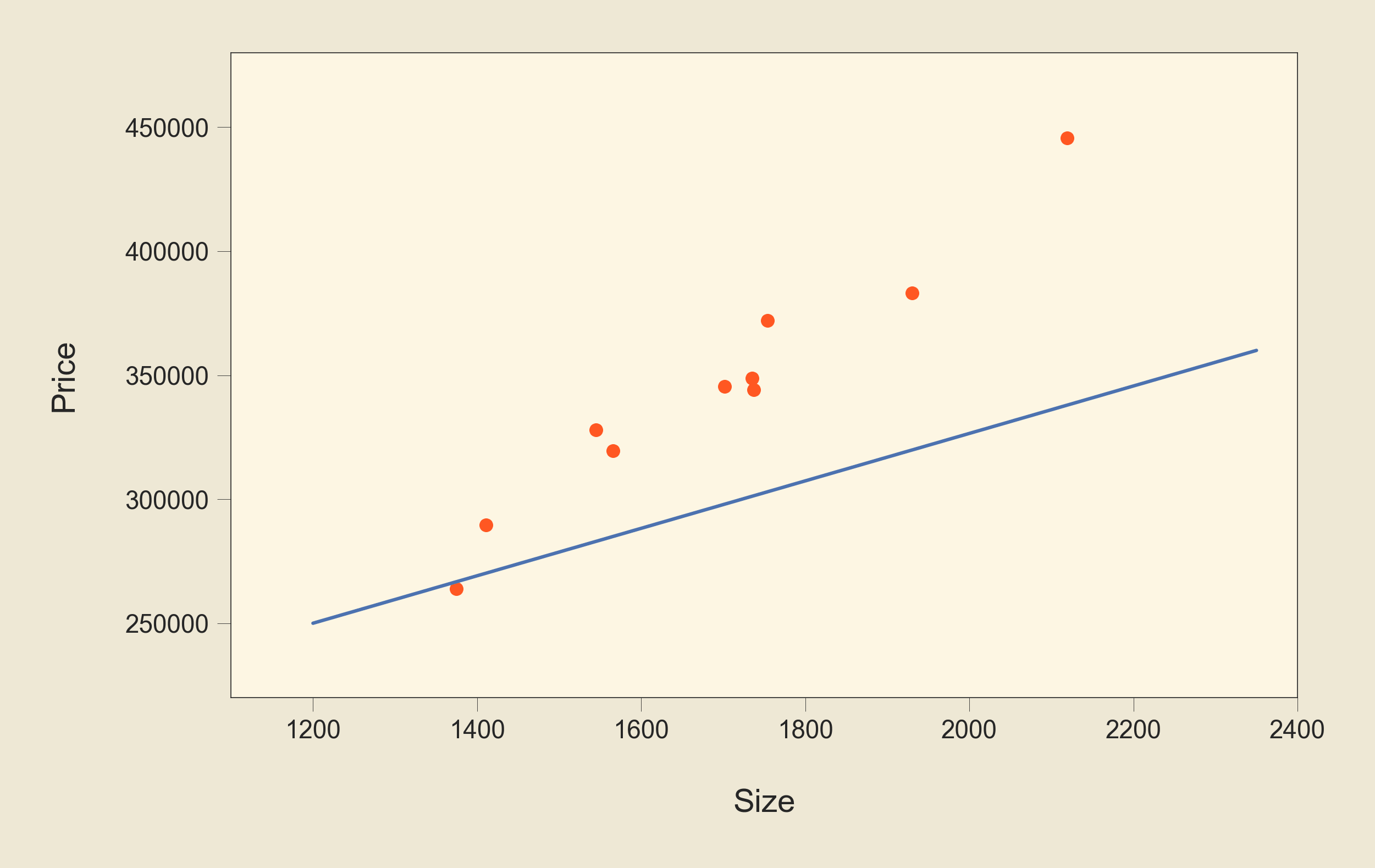
This one is better but still not good enough. Let's write a simple Python code using scikit-learn library, which is a great Python library that allows us to build many machine-learning models easily with a few lines of code:
# import the part that we need from scikit-learn
from sklearn.linear_model import LinearRegression

# Create the features array.
# We have one feature in our example =>
# one column in feature array
x = [[1375],
[1737],
[1702],
[1411],
[2119],
[1735],
[1545],
[1566],
[1754],
[1930]]

# Create the target array
y = [263928,
344085,
345505,
289701,
445548,
348764,
328066,
319531,
372130,
383157]

# Create an instance of LinearRegression model
model = LinearRegression()

# Fit the model to our data with one command
model.fit(x, y)

# Now we can see the value of the parameters
# theta_0 and theta_1
# theta_0 is stored in model.intercept_
print("theta_0 =", model.intercept_)
# -22610.91211103683
# theta_1 is stored in model.coef_
print("theta_1 =", model.coef_)
# [217.28837982]
When we run these lines of code, we get the values of \(\theta_0\) and \(\theta_1\):
theta_0 = -22610.91211103683
theta_1 = [217.28837982]
Now that we have the optimal values for our parameters, let's plot the line using these values:
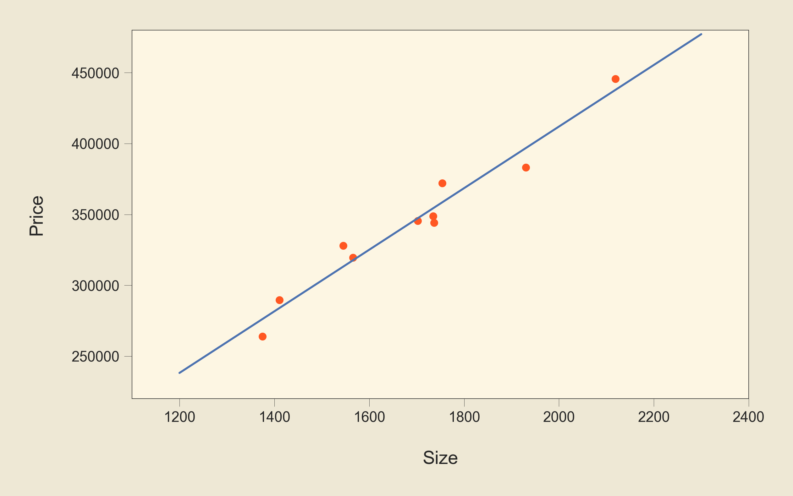
We can see that this line represents a better fit to the data than the previous two lines. And now, we can use the equation of this line that we talked about earlier:
$$ h_\theta(x)=\theta_0+\theta_1x $$
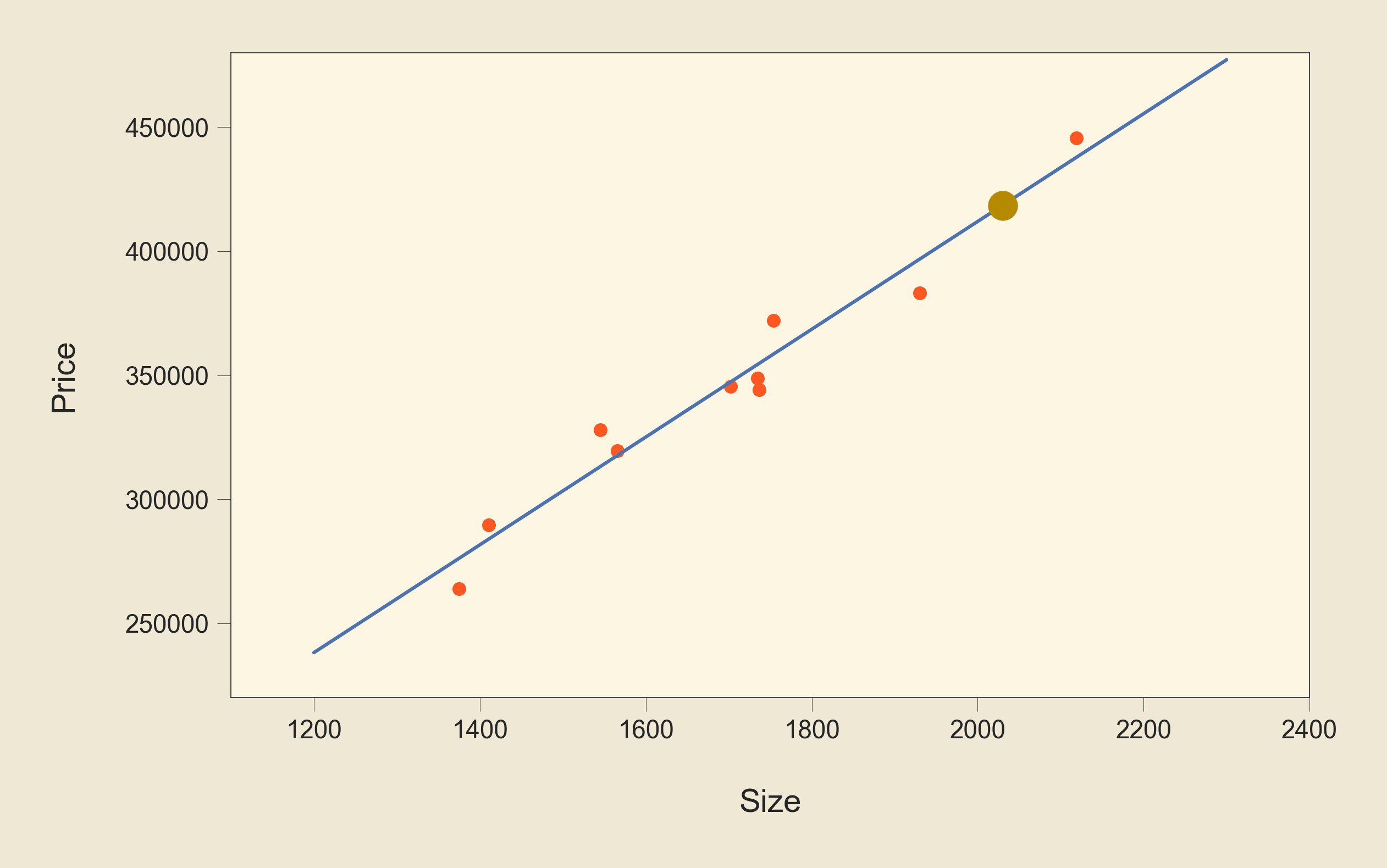
to predict the output for new data. Let's have an example: suppose that we get a new data, which is the size of a house, and we want to predict its price using our model. If the size is 2030 m2. We can calculate the predicted values as follows:
$$ h_\theta(2030)=-22610.91211103683+217.28837982\times2030\\~\\=418484.49892356317 $$
So the predicted price is $418484.5. We can get the same value using the model that we built in Python:
print(model.predict([[2030]]))
This would be the new data point that we just predicted its target value; it is shown in yellow:
This post is highly influenced by Machine Learning course by Prof. Andrew Ng.
